
Introduction
There is a question every safety-critical software engineer has asked at some point: is it possible to prove that a program will never access an array out of bounds, never divide by zero, never dereference a null pointer — without running the program against every possible scenario?
The answer, within certain limits, is yes. The underlying theory is called abstract interpretation, formalized by Patrick and Radhia Cousot in 1977. It's the same theory behind the analyzers used today in avionics, automotive, and railway signaling — domains where a runtime error isn't a bug, it's an incident.
In this article we open the black box: how the program is turned into a graph, how an engine walks that graph maintaining a table of approximations, and how small verifiers use that table to decide, at every critical operation, whether there's a risk of error.
1 — The core idea: running the program in an approximated world
Actually executing a program means picking concrete values for its inputs and following a single execution path at a time. To prove a property for every possible input, you'd need to repeat that infinitely many times.
Abstract interpretation solves this by replacing concrete values (e.g. x = 7) with abstract values that represent an entire set of possibilities (e.g. x ∈ [0, 10]). Instead of simulating one execution at a time, the analyzer simulates all executions at once, approximately.
That approximation has to respect a golden rule called soundness: the abstract set must necessarily contain every concrete value the program can actually take at that point. It may contain more than that (over-approximation), but never less.
2 — The control flow graph (CFG)
Before propagating anything, the code needs to be turned into a structure the analysis can actually walk: the Control Flow Graph (CFG).
Each node in the CFG represents a basic block — a sequence of instructions with no internal branching — and each edge represents a possible transfer of control: an if, a while, a function call, a goto. Points where two or more edges meet are called join points, and they are exactly where the analysis needs to combine information coming from different paths.
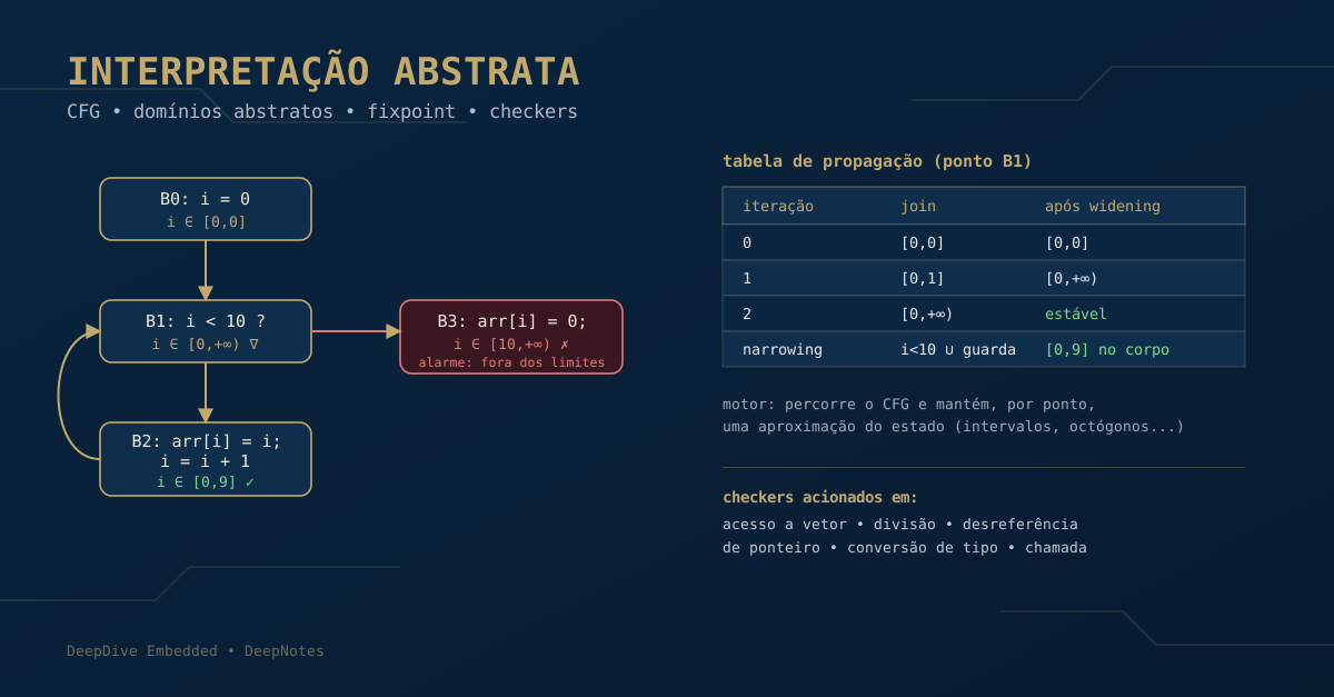 CFG of a classic loop: the engine propagates intervals block by block, and the checker flags the out-of-bounds access in B3.
One detail that's easy to miss: loops create cycles in the CFG. That means computing the abstract state of a block inside a loop requires first knowing the state of the loop itself — a circular dependency. This is exactly the problem the propagation engine solves by iterating up to a fixpoint.
3 — Abstract domains: intervals, octagons, and everything in between
The abstract domain defines what shape the approximation can take. It's the single most important design decision in any analyzer, because it trades precision against computational cost.
-
Interval domain: each variable gets a pair
[min, max], independent of the others. It's cheap — linear cost in the number of variables — but non-relational: it can't express thaty = x + 1, for instance. It loses precision whenever one variable's behavior depends on another's. -
Octagon domain: keeps constraints of the form
±x ± y ≤ cbetween pairs of variables. It's weakly relational — it can capture relations like "the index never exceeds the array size minus one" — with quadratic cost (O(n²) constraints for n variables), still tractable for real code. - Polyhedral domains: arbitrary linear constraints across multiple variables. Much more precise, but with worst-case exponential cost — rarely applied to an entire program, only to small, critical fragments.
4 — The propagation engine: how the state table is built
The heart of the analysis is an algorithm that walks the CFG and maintains, for every point in the program, a table mapping each variable to its current abstract value. In practice, it works like a worklist:
- Every block in the CFG starts with the abstract state empty (no information yet, or "unreachable").
- The engine processes one block at a time, applying the transfer function of each instruction to the incoming state — for example, for
i = i + 1withi ∈ [0,5], the output isi ∈ [1,6]. - When a block has more than one predecessor (a join point), the engine combines the states coming from each path with a join operation — for intervals, that's simply the smallest minimum and the largest maximum between the two sides.
- The result is propagated to the following blocks, and the process repeats until the table stops changing — the so-called fixpoint.
The problem is that, inside a loop, the join tends to grow with every iteration ([0,0], then [0,1], then [0,2]...) and would never stabilize on its own in finite time. To force convergence, the engine applies a widening operator (∇): instead of precisely summing bounds step by step, it "jumps" straight to a wider bound (for example +∞, or a constant already seen in the code as a comparison value).
This guarantees termination, but usually loses precision. That's why, once widening has stabilized the analysis, the engine runs a second phase called narrowing (∆): it reapplies the transfer functions (without widening again) to "tighten" the result and recover part of the lost precision, without ever violating soundness.
Here's how that looks in a real table, for the loop below:
int arr[10];
int i = 0;
while (i < 10) {
    arr[i] = i;      // B2
    i = i + 1;
}
arr[i] = 0; // B3 -- classic off-by-one bug| Iteration (point B1) | Plain join | After widening / narrowing |
|---|---|---|
| 0 (entry) | i ∈ [0,0] | i ∈ [0,0] |
| 1 | i ∈ [0,1] | i ∈ [0,+∞) (widening) |
| 2 | i ∈ [0,2] | stable — fixpoint reached |
narrowing + guard i<10 |
— | inside the loop: i ∈ [0,9] |
| loop exit (B3) | — | i ∈ [10,+∞) |
i ∈ [0,9] combined with the guard i<10 shows the access at B2 is safe. But at B3, outside the loop, the propagated state is i ∈ [10,+∞) — the smallest possible value already equals the array size. The access arr[i] at B3 is guaranteed to be out of bounds.
5 — Checkers: where theory becomes an alarm
The propagation engine, on its own, doesn't know what "an error" is. It only keeps the state table up to date. The ones interpreting that table are the checkers — small verifiers attached to the language operations that can fail at runtime:
- Array access: the checker looks up the index's interval and checks whether it's contained in
[0, size-1]. - Division: the checker checks whether the divisor's interval excludes zero.
- Pointer dereference: the checker checks whether the pointer's abstract value excludes null (or known invalid addresses).
- Type conversion: the checker checks whether the source interval fits within the destination type's range (for example, a 32-bit
intconverted to an 8-bitchar). - Function call: the checker checks whether the arguments satisfy the preconditions expected by the called function (or its summary, if the analysis is modular).
The important part is that checkers don't re-analyze anything. They only trigger at these critical operations and simply query the abstract state the engine has already computed at that exact point in the CFG. If the state proves the operation is safe, nothing happens. If the state cannot prove safety, the checker raises an alarm — which may be a real bug or a false positive, but never a false negative, thanks to the soundness of the analysis.
6 — Optimizations used in practice
Applied naively to a real program, the pure theory of abstract interpretation would be far too slow and far too imprecise. Real analyzers apply several optimizations to make it tractable:
-
Widening with thresholds: instead of jumping straight to
+∞, widening jumps to constants that already appear in the source code (loop bounds, comparisons, buffer sizes). This dramatically reduces the precision loss without compromising termination. - Delayed widening: the first few iterations of a loop use a plain join, and widening only kicks in after some rounds — giving the analysis time to "feel out" the real growth pattern of the variable before widening it.
- Variable packing: in relational domains like octagons, tracking relations between every variable in the program is infeasible. Analyzers group only the variables that actually appear together in expressions (indices and sizes of the same array, for instance), reducing the cost from a global O(n²) to several small groups.
- Reduced product of domains: combining a cheap domain (intervals) with a more expensive, specific one (congruences, octagons) only where needed, exchanging information between them to gain precision without paying the expensive domain's cost across the whole program.
- Modular analysis via function summaries: instead of re-analyzing an entire function's body every time it's called, a summary is computed once (the relation between the parameters' preconditions and the return's postconditions) and reused at every call site.
-
Trace partitioning: at join points where merging the states would lose important information (for example, after an
ifwhose branches behave very differently), the analysis keeps the states separate for a while, delaying the join to a point where the precision loss is less costly.
All of these techniques follow the same principle: spend computational precision only where it changes the result. It's this balance — not the sophistication of the abstract domain in isolation — that decides whether an analyzer can run on a codebase of hundreds of thousands of lines in a viable amount of time.
7 — Why this matters in critical systems
In critical embedded software — flight control, automotive powertrain, railway signaling — an undetected runtime error might only manifest under a combination of conditions that's practically impossible to reproduce on a test bench. This is exactly the kind of analysis that made it possible, for example, to formally prove the absence of runtime errors in Airbus flight control software, covering properties such as arithmetic overflow, division by zero, and invalid array access — something no test suite, however extensive, can guarantee with mathematical certainty.
The value of abstract interpretation isn't to replace testing — it's to prove, with mathematical guarantees, the absence of entire classes of errors that testing could never fully cover.
Conclusion
Behind any serious static analyzer sits the same machinery: a CFG that structures the program, a propagation engine that walks that graph maintaining a table of approximations per abstract domain, and checkers that query that table at the points where the language can fail at runtime. Widening and narrowing exist to guarantee all of this terminates in finite time without giving up soundness; the packing, threshold, and summary optimizations exist so that this mathematical guarantee is actually achievable on real code, not just textbook examples.
Main Takeaway
Abstract interpretation isn't magic, and it isn't "an AI that understands code" — it's lattice and fixpoint mathematics applied in a disciplined way to a program's control flow.
Understanding the CFG, the abstract domains, and the split between engine and checkers is what lets you read the result of any static analysis with the right eyes: an alarm isn't necessarily a bug, but the absence of an alarm, in a sound analysis, is a guarantee.
References
-
Cousot, P., Cousot, R.
Abstract Interpretation: A Unified Lattice Model for Static Analysis of Programs by Construction or Approximation of Fixpoints.
POPL, 1977.
The founding paper of abstract interpretation: lattices, approximation, and fixpoint computation. -
Cousot, P., Cousot, R.
Comparing the Galois Connection and Widening/Narrowing Approaches to Abstract Interpretation.
PLILP, 1992.
Formalizes the widening and narrowing operators used to guarantee termination on loops. -
Miné, A.
The Octagon Abstract Domain.
Higher-Order and Symbolic Computation, 2006.
Defines the octagon domain, the basis for relational analyses with quadratic cost. -
Blanchet, B. et al.
A Static Analyzer for Large Safety-Critical Software.
PLDI, 2003.
Describes the architecture of an abstract-interpretation analyzer applied to large-scale C code. -
Souyris, J. et al.
Establishing the Absence of Run-Time Errors and Undefined Behaviour in Airbus Flight Control Software.
Case study on applying abstract interpretation to critical flight control software. Available at: https://www.astree.ens.fr/papers/astree_airbus_sas2007.pdf . -
Nielson, F., Nielson, H. R., Hankin, C.
Principles of Program Analysis.
Springer, 1999.
A comprehensive textbook reference on data-flow analysis, CFGs, and abstract domains.

Comments and discussion